Challenge

Main Goal

The goal of this competition is to propose new and fast star identification algorithms for star trackers that are robust to measurement uncertainties and artifacts. Given only one image as information, this scenario models a spacecraft being "lost in space", which means that there is no prior information on the spacecraft's orientation. It is your job to recover a sense of orientation allowing the spacecraft to keep pursuing the goal of its mission.

In a nutshell

Star trackers are devices commonly present in most spacecraft to determine orientation based on camera images of stars.

A crucial element of the star tracker functioning is the star identification algorithm. This algorithm is presented with an image containing spikes (bright points) that can represent either true stars or artifacts. Using a catalog of stars defined by an identifier \(h\), a magnitude \(m\) and by two angles \(\omega, \psi\) determining their position on the galactic sphere, the star identification algorithm maps each of the spikes to an appropriate star in this catalog or classifies it as an artifact. The input to the algorithm (a scene) is thus a set of \(N\) image coordinates and magnitudes \(C = \{[x_1\ y_1\ m_1], [x_2\ y_2\ m_2], ..., [x_N\ y_N\ m_N]\}\) and the output is a set of identifiers \(H = \{h_1, h_2, ..., h_N\}\) from the catalog (false stars will be identified by a default identifier \(h_F\)). The star identification algorithm can therefore be seen as a function \(H = f(C)\).

In this competition, a star catalog is given (see the data page), together with a large number of possible scenes \( C_i, i = 1 .. N\) and the participants are asked to submit a file containing the identification made for all stars in each scene, and optionally a separate C file containing their code as to allow us to profile it.

Scene generation

Understanding how a scene is generated helps helps to identify stars in a scene. In other words, how does a given star end up as a spike in some image position? This process is, essentially, the inverse of star identification. The implementation of our scene generation can be found on the scripts page and you can use it to create your own scenes. The code is only provided as a courtesy and it is not necessary for the purpose of submitting a solution to the problem, but it certainly helps in understanding it in case of non experts. The parts of the code (simulator.py) that implement the described formulas are explicitly referenced.

Understanding the camera model

We are given the star's identifier \(h\) and want to know its coordinates (if any) \(x\) and \(y\) in the image of our star tracker camera. The first step is to determine the position of the star in the celestial sphere. While the stars have different distances from our solar system, one can consider all stars to be infinitely far away. Therefore, two angles are enough to describe the position of the star on the celestial sphere. The star catalog contains the right ascension \(\omega\) and declination \(\psi\) of the star in the International Celestial Reference System (ICRS J1991.25). Figure 1 shows a hemisphere of the celestial sphere with the cardinal points (N, E, S, W) and the zenith (Z). The right ascension is the angle between the north point and the stars position projected on the horizontal plane. This angle can be between 0 and 360 degrees and corresponds to a rotation around the z-axis. The declination then is the angle between the horizontal plane and the actual star. To get to the zenith (top) of the sphere, this angle has to be 90 degrees, or -90 to reach the nadir (bottom), so the angle can be between -90 and 90 degrees. The right ascension and declination are stored next to the HIP number (star identifier) in the star catalog implemented in the StarCatalog class, that loads the catalog data.

The next step is to transform this position of the star in the galactic coordinate system to the image coordinate system. To do so, a model of the camera is used consisting of an extrinsic and intrinsic part. The extrinsic part describes the outer transformation of the star position as seen in the celestial reference frame to the camera/observer reference frame. Typically the location and orientation and in our case reduced to just the orientation. The intrinsic part describes the transformation done by the optical system of the camera and for example contains the distortion caused by the lens. It transforms the observer reference frame coordinates to the image plane coordinates.

Extrinsic model

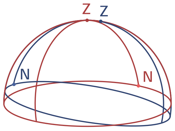
The camera can have any arbitrary orientation with respect to the celestial reference frame. The camera/observer reference system has its own cardinal points (N, E, S, W) which are more commonly called up, right, down and left, as well as zenith (front) and nadir (back). Figure 2 illustrates this point of view: the celestial reference frame is shown in red and the camera reference frame is illustrated in blue. There are several options to transform the angles in the celestial reference frame \(\omega\) and \(\psi\) into the frame of the camera. One way is to transform the angular representation into a unit-vector and use a rotation matrix or quaternions to rotate them, before transforming them back into an angular representation. We call the angular representation that we obtain this way as azimuth and altitude, which correspond to the right ascension and declination in the original galactic coordinate system. To not introduce too many variables we will keep the notation \(\omega\) and \(\psi\) for azimuth and altitude respectively from now on.

The implementation contains the functions angles_to_vector and vector_to_angles to transform from angle to vector representation and vice versa. The transformation itself is done with a rotation matrix that can simply be multiplied with numpy's dot function. Two functions help to generate such a rotation matrix: lookat creates a rotation matrix that makes the camera look at a specific direction in the celestial reference frame and random_matrix creates a random rotation matrix.

Intrinsic model

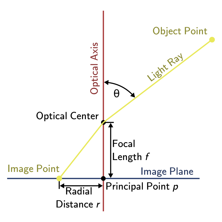
Figure 3 shows a side view of the intrinsic camera model. The camera projects the light onto the image plane. The incoming lightray passes through the optical center. The optical axis is the axis that is normal to the image plane and passes through the optical center. The incoming ray comes at an angle \(\theta = \frac{pi}{2} - \psi\) to the optical axis and passes through the optical center where it is distorted. We assume this distortion to be radially symmetric, so the azimuth of the incoming ray is not distorted. The principal point \(p\) is the point on the image where the optical axis and image plane intersect. Ideally this would be the center of the image.

The radial distance \(r\) from the principle point is a function of the angle \(theta\). For an undistorted lightray that passes the optical center without a change of direction, this function is

$$r(\theta) = f \tan(\theta),$$

where \(f\) is the focal length. This model is known as the rectilinear or perspective camera model. Other commonly used projection functions are the (1) stereographic, (2) equidistant or equi-angular, (3) equisolid angle or equal area, and (4) orthographic projection:

$$\begin{align} r_1(\theta) &= 2f \tan\left(\frac{\theta}{2}\right) \\ r_2(\theta) &= f \theta \\ r_3(\theta) &= 2f \sin\left(\frac{\theta}{2}\right) \\ r_4(\theta) &= f \sin(\theta) \end{align}$$

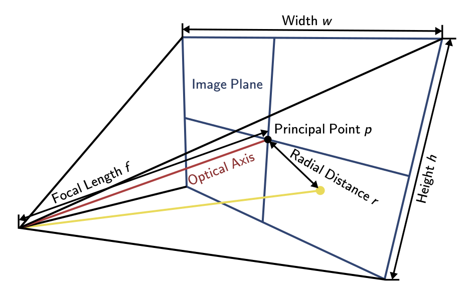
Figure 4 shows the intrinsic camera model from a different perspective. We can see the width \(w\) and height \(h\) of the image. Using the equation for the rectilinear projection, we can also determine the field of view \(fov_x\) in the x-direction as

$$fov_x = 2 \tan^{-1}\left(\frac{w}{2 f}\right),$$

where the focal length \(f\) is given in pixels. If the focal length is given in meters another factor comes into play, which is the pixel size \(s\) on the sensor given in meters. Note that in case of non-square pixels, the focal length in pixels differs for the x- and y-axis. This is typically considered by using the focal length for the x-axis and multiplying \(r\) by the pixel size aspect ratio for the y-axis.

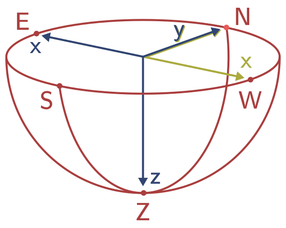
A final step we have to consider is the coordinate system of our image. Previously we defined the camera to look into the positive z-axis direction and the positive y-axis is up. In our right-handed coordinate system this results into the x-axis pointing left instead of the usual right as we want to have it in our image. This is illustrated in figure 5, where the hemisphere has been turned around, so that you can imagine the image lying on the base of the hemisphere, as if it would lie on a table. The original three-dimensional axes are colored blue, while the target two-dimensional image axes are colored in yellow. One way to solve this problem is to simply flip the x-axis. Alternatively we can also transform the azimuth \(\omega\) to the angle \(\alpha = \pi - \omega\).

Now we can combine all these efforts into our final equations:

$$\begin{align} x &= r(\theta) \cos(\alpha) + p_x\\ y &= \frac{s_x}{s_y} r(\theta) \sin(\alpha) + p_y \end{align}$$

The intrinsic camera model is implemented in the abstract class Camera with derivative classes implementing the different projection functions (RectilinearCamera, EquidistantCamera, OrthographicCamera, etc.). The Camera class offers two methods: from_angles transforms from angles to pixel coordinates and to_angles transforms in the opposite direction.

Star Magnitude

The magnitude of a star has been historically measured on a relative logarithmic scale. The brightest stars were given a magnitude of 1 and the most faint stars that were still visible by eye a magnitude of 6. Magnitude was assigned based on comparison with other stars. Due to the eyes' logarithmic sensitivity, the magnitude is logarithmically related to the luminous intensity. Today the magnitude is calibrated based on a set of reference stars. Per definition, 5 magnitude steps correspond to a factor 100 difference in luminous intensity. This definition leads to the formula

$$m - m_{ref} = -2.5 \log\left(\frac{I}{I_{ref}}\right),$$

where \(m\) is the magnitude and \(I\) is the luminous intensity. For example a star with a magnitude \(m = 5\) compared to a reference star with \(m_{ref} = 0\) leads to

$$\frac{I}{I_{ref}} = 10^{\frac{5 - 0}{-2.5}} = 10^{-2} = \frac{1}{100},$$

as expected from the definition.

A star tracker camera can then be calibrated by measuring reference stars with known magnitude. The number of photoelectrons that are measured by the sensor are assumed to be proportional to the luminous intensity. The problem in practice is of course noise, which will be discussed in the next section.

Noise

Real star tracking systems deal with different sources of noise. In general, the noise on the position \(x\) and \(y\) is lower than on the magnitude \(m\). For this reason some star tracker algorithms completely ignore the magnitude information. The centroiding of the stars in practice is more accurate than the quantization noise of a single pixel. The centroiding noise is modeled as a Gaussian noise.

The magnitude has different types of noise contributions, such as dark current, shot noise and readout noise. Overall the noise components on the magnitude are modelled with different contributions from Poisson, Gaussian and other types of noise. These noise components on the magnitude are modeled in the class StarDetector.

Finally, the noise might cause the centroiding algorithm to not discover stars or detect artifacts. Reflections or radiation can cause the camera to detect spikes that are not actual stars. The star identification algorithm has to deal with these artifacts and mark them as such.

The overall scene generation is implemented in the Scene class. The static method random generates a random scene calling the methods compute computing a random orientation, transforming the celestial coordinates to the image plane and adding the Gaussian centroiding noise to this possion, add_false_stars which adds a random number of artifacts, scramble scrambling the order of the stars and artifacts in the scene and finally add_magnitude_noise adding the magnitude noise modeled with the StarDetector class. The method render can be used to visualize the image that the star tracker camera would see.